Microscopy, Python, and Open Source: Perfecting the Details
.webp)

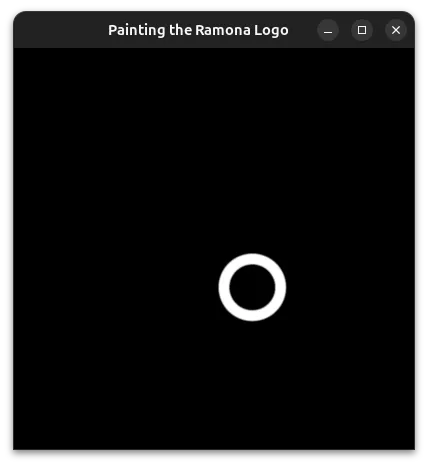
This is Part 2 of our blog series on creating a pixel-perfect logo using Python and open source tools. If you haven't already, check out Part 1: From Pixels to Infinity where we introduce signed distance fields (SDFs) and tackle the basic circles and ring components of the Ramona logo.
In Part 1, we redrew the Ramona logo with a mathematically precise signed-distance field (SDF) so it stays crisp at any zoom. We covered the basics of SDFs and tackled the three circles and ring components.
Now in Part 2, we'll tackle the more challenging circle connectors, complete the outer perimeter, and show how everything combines into a pixel-perfect logo that works beautifully with gigapixel microscopy data.
The circle connectors
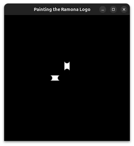
The small circle connectors in our logo were quite challenging for me to define mathematically. In one approximation, we can take the connections to be the empty spaces between circles that are tangent to the original 3 circles. My inspiration came from looking at coins on my desk.
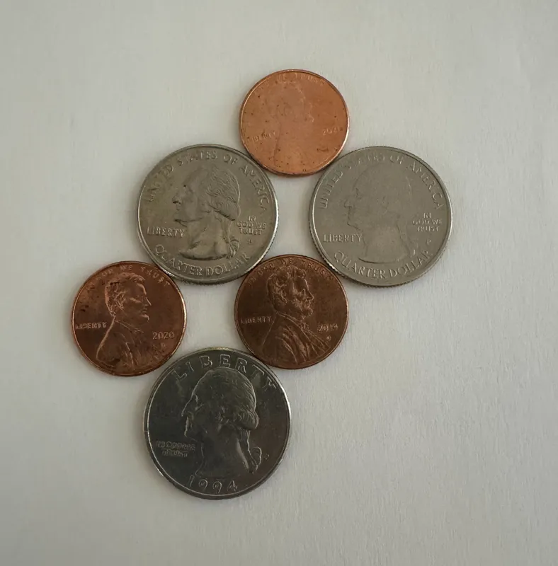
If the coins are of correct size, and appropriately arranged, then they start to resemble the 3 connected circles. However, before we proceed, we want to find a mathematical relationship between the circles as a function of their radius, the gap between adjacent circles, and the width of the connector at its narrowest point. This took me back to high school algebra!

Taking our two formulas:

Along with the identity,
.webp)
We find the final relationship:
.webp)
We can use this to draw an attempt of our concept on the screen.
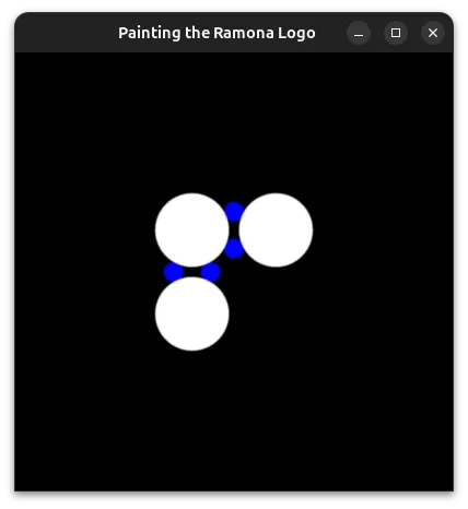
Unlike our toy example with coins, here we needed to draw 4 blue circles to define a proportionally sized gap for our connecting lines.
let coord_use = coord / size * 2;
let thickness = 0.1;
let thickness_half = 0.05;
let radius = 1. / 3.;
let gap = 0.05;
let circle_offset = radius + gap;
let teardrop_gap = 1. / 12.;
let connecting_circle_radius = {a};
let tiny_circle1 = length(coord_use - vec2<f32>(-circle_offset + teardrop_gap + connecting_circle_radius, 0.)) - connecting_circle_radius;
let tiny_circle2 = length(coord_use - vec2<f32>(-circle_offset - teardrop_gap - connecting_circle_radius, 0.)) - connecting_circle_radius;
let tiny_circle3 = length(coord_use - vec2<f32>(0., circle_offset + teardrop_gap + connecting_circle_radius)) - connecting_circle_radius;
let tiny_circle4 = length(coord_use - vec2<f32>(0., circle_offset - teardrop_gap - connecting_circle_radius)) - connecting_circle_radius;
let tiny_circles_left = min(tiny_circle1, tiny_circle2);
let tiny_circles_top = min(tiny_circle3, tiny_circle4);
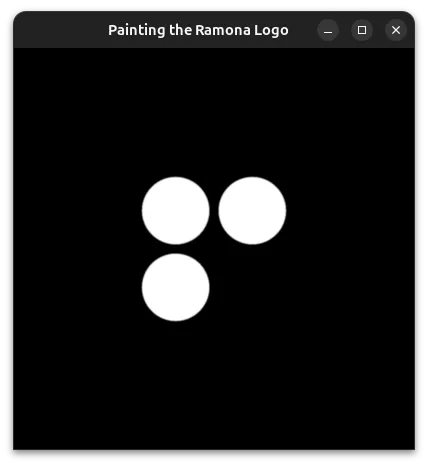
return min(tiny_circles_top, tiny_circles_left) * size;We will then want to define a bound for the gap to fill. To help us debug, we'll draw this as a rectangle with a red color. The order in which we draw things is important, and therefore we start by drawing the white circles, followed by red rectangles to fill in the gaps, and finally by blue circles that cover the regions of the red rectangles we want to hide.
We can now take the union of the red and white areas, and subtract the blue circles. We follow the operators defined in Rougier's paper and obtain:
return max(min(three_circles, tiny_rectangles), -tiny_circles);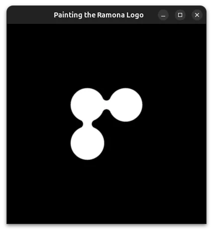
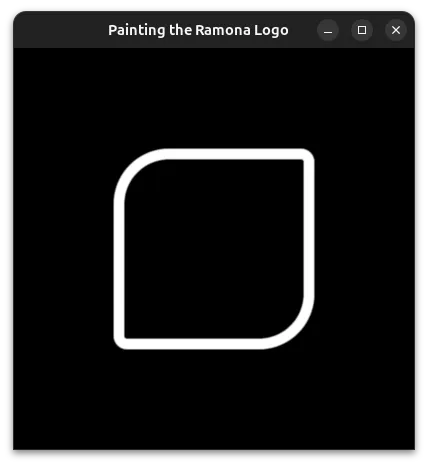
The outer perimeter
We will begin by using the formula for a square for the outer perimeter. For this we will use Inigo Quilez's (IQ) formula for a Rounded Box. We'll combine this with IQ's formula to make any one of his SDFs annular.
from wgpu.gui.auto import WgpuCanvas, run
import pygfx as gfx

custom_sdf = """
    let coord_use = coord / size * 2;
    let thickness = 0.1;
    let thickness_half = 0.05;

    let bounds = vec2<f32>(1.0) - thickness_half;

    let roundness = vec4<f32>(0.08, 0.5, 0.5, 0.08);
    let roundess2 : vec2<f32> = select(roundness.xy, roundness.zw, coord_use.x > 0.);
    let r = select(roundess2.x, roundess2.y, coord_use.y > 0.);

    let q = abs(coord_use) - bounds + r;

    let rounded_rectangle = min(max(q.x,q.y),0.0) + length(max(q, vec2<f32>(0.0))) - r;
    let outer_square = abs(rounded_rectangle) - thickness_half;

    return outer_square * size;
"""

scene = gfx.Scene()
scene.add(gfx.Background.from_color("#000", "#000"))

point = gfx.Points(
    gfx.Geometry(positions=[[0, 0, 0]]),
    gfx.PointsMarkerMaterial(
        size=200,
        size_space='world',
        marker="custom",
        edge_width=0,
        custom_sdf=custom_sdf,
    ),
)
scene.add(point)

canvas = WgpuCanvas(title="Painting the Ramona Logo", size=(400, 400))
renderer = gfx.WgpuRenderer(canvas)
camera = gfx.OrthographicCamera(400, 400)
controller = gfx.PanZoomController(camera, register_events=renderer)
canvas.request_draw(lambda: renderer.render(scene, camera))

if __name__ == "__main__":
    run()
The beauty of this implementation compared to a traditional image of finite resolution is that it makes beautiful shapes no matter how much you decide to zoom in!!!

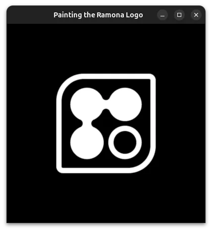
Combining it all
Now that we have SDFs for all the parts of our logo, we can combine them by taking the minimum distance of all 4 individual components.

Gigapixel Microscopy Challenges
One challenge particular to Ramona's logo in the user interface is that we would like it to look amazing whatever you place under the microscope. This is where Pygfx shines in that it allows us to have transparency built into the display pipeline! However, in the examples above we assumed we have a perfectly black background. We would want to consider how the logo might look on a lighter background which can occur if you are looking at your samples under brightfield illumination. A popular strategy is to draw an outline for the logo.
However, with the thin lines and small gaps, a typical outline starts to look awkward when the logo becomes smaller. Instead we are opting to fill the inner region of the logo with a semi-transparent layer. For this we will reuse the same SDF that we used for the perimeter, but without the annular feature. We will add this as a point "behind" the rest of the logo and allow Pygfx to render it all for us live!
We can preview what the results look like when we add a background of "#00000033" (black, 20% opacity) to our logo under a background defined by a gradient.

With the mathematically exact definition for the Ramona Logo, we can display and interact with it at various scales without affecting the quality of the symbol or your images.
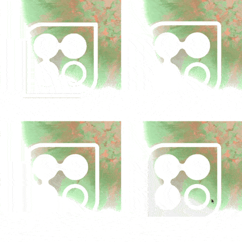
For one final look at the before, after let's look at the different implements altogether. On the top left, we show on the top left a typical PNG of a logo (128 x 128 pixels). On the top right, we show the SDF implementation we described in the post. On the bottom left, we compare it to the exact SDF of our logo; however, the construction of an exact SDF is significantly more complicated. The results between the approximate SDF and the closed-form solution seem indistinguishable. On the bottom right, we add a dark transparent fill to the logo to make it more visible on white backgrounds. In the animation, show how the logo appears on real microscopy data where colors can vary widely, especially when considering both brightfield and fluorescence images. On the bottom right, the semidark transparent fill helps one see the logo even in the presence of a white image.
Can I use this in my project?
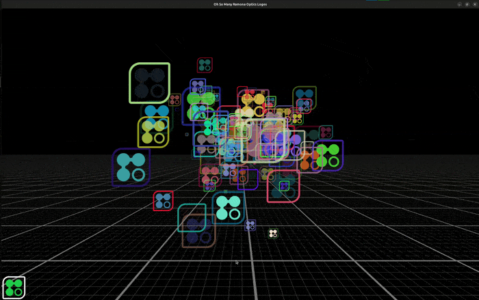
To draw our logo, we leveraged some new features of Pygfx that should be available on the release after 0.3.0, see GitHub pull request 822. If your logo or icon cannot be described as a signed distance field, Almar and the Pygfx team have enabled you to define it as an image since version 0.3.0 which can be installed either through pip or conda! If one logo and a single color feel limiting to you, don't worry, Pygfx provides you with the capabilities of a 3D engine enough to add as many logos in as many colors as your heart desires.
While displaying logos may not sound like the most mission critical task, ensuring proper display of image data as well as labels and annotations is critical to improving how we communicate science as a whole. Hopefully you find this little technical demonstration fun and inspiring! It would be foolish to write from scratch every single line of code we make use of at Ramona. We believe that by working with the open source community, we can leverage the work of many expert programmers and scientists before us and contribute back to the community at large to provide you with the best gigapixel microscopy experience!
Footnote: The exact SDF has a few properties that make it more amenable to drawing edges and contours, however, it is significantly more complicated to write out mathematically and so we leave it as an exercise to the interested readers. We point readers to a blog post from IQ that describes some of the advantages of exact SDFs https://iquilezles.org/articles/interiordistance/. Even without an exact SDF one can still draw pixel perfect shapes albeit without an adjustable outline thickness!
This is Part 2 of our blog series on creating a pixel-perfect logo using Python and open source tools. If you haven't already, check out Part 1: From Pixels to Infinity where we introduce signed distance fields (SDFs) and tackle the basic circles and ring components of the Ramona logo.
In Part 1, we redrew the Ramona logo with a mathematically precise signed-distance field (SDF) so it stays crisp at any zoom. We covered the basics of SDFs and tackled the three circles and ring components.
Now in Part 2, we'll tackle the more challenging circle connectors, complete the outer perimeter, and show how everything combines into a pixel-perfect logo that works beautifully with gigapixel microscopy data.
The circle connectors
The small circle connectors in our logo were quite challenging for me to define mathematically. In one approximation, we can take the connections to be the empty spaces between circles that are tangent to the original 3 circles. My inspiration came from looking at coins on my desk.
If the coins are of correct size, and appropriately arranged, then they start to resemble the 3 connected circles. However, before we proceed, we want to find a mathematical relationship between the circles as a function of their radius, the gap between adjacent circles, and the width of the connector at its narrowest point. This took me back to high school algebra!
Taking our two formulas:
Along with the identity,
We find the final relationship:
We can use this to draw an attempt of our concept on the screen.
Unlike our toy example with coins, here we needed to draw 4 blue circles to define a proportionally sized gap for our connecting lines.
let coord_use = coord / size * 2;
let thickness = 0.1;
let thickness_half = 0.05;

let radius = 1. / 3.;
let gap = 0.05;
let circle_offset = radius + gap;
let teardrop_gap = 1. / 12.;
let connecting_circle_radius = {a};

let tiny_circle1 = length(coord_use - vec2<f32>(-circle_offset + teardrop_gap + connecting_circle_radius, 0.)) - connecting_circle_radius;
let tiny_circle2 = length(coord_use - vec2<f32>(-circle_offset - teardrop_gap - connecting_circle_radius, 0.)) - connecting_circle_radius;
let tiny_circle3 = length(coord_use - vec2<f32>(0., circle_offset + teardrop_gap + connecting_circle_radius)) - connecting_circle_radius;
let tiny_circle4 = length(coord_use - vec2<f32>(0., circle_offset - teardrop_gap - connecting_circle_radius)) - connecting_circle_radius;

let tiny_circles_left = min(tiny_circle1, tiny_circle2);
let tiny_circles_top = min(tiny_circle3, tiny_circle4);

return min(tiny_circles_top, tiny_circles_left) * size;
We will then want to define a bound for the gap to fill. To help us debug, we'll draw this as a rectangle with a red color. The order in which we draw things is important, and therefore we start by drawing the white circles, followed by red rectangles to fill in the gaps, and finally by blue circles that cover the regions of the red rectangles we want to hide.
We can now take the union of the red and white areas, and subtract the blue circles. We follow the operators defined in Rougier's paper and obtain:
return max(min(three_circles, tiny_rectangles), -tiny_circles);The outer perimeter
We will begin by using the formula for a square for the outer perimeter. For this we will use Inigo Quilez's (IQ) formula for a Rounded Box. We'll combine this with IQ's formula to make any one of his SDFs annular.
from wgpu.gui.auto import WgpuCanvas, run
import pygfx as gfx

custom_sdf = """
    let coord_use = coord / size * 2;
    let thickness = 0.1;
    let thickness_half = 0.05;

    let bounds = vec2<f32>(1.0) - thickness_half;

    let roundness = vec4<f32>(0.08, 0.5, 0.5, 0.08);
    let roundess2 : vec2<f32> = select(roundness.xy, roundness.zw, coord_use.x > 0.);
    let r = select(roundess2.x, roundess2.y, coord_use.y > 0.);

    let q = abs(coord_use) - bounds + r;

    let rounded_rectangle = min(max(q.x,q.y),0.0) + length(max(q, vec2<f32>(0.0))) - r;
    let outer_square = abs(rounded_rectangle) - thickness_half;

    return outer_square * size;
"""

scene = gfx.Scene()
scene.add(gfx.Background.from_color("#000", "#000"))

point = gfx.Points(
    gfx.Geometry(positions=[[0, 0, 0]]),
    gfx.PointsMarkerMaterial(
        size=200,
        size_space='world',
        marker="custom",
        edge_width=0,
        custom_sdf=custom_sdf,
    ),
)
scene.add(point)

canvas = WgpuCanvas(title="Painting the Ramona Logo", size=(400, 400))
renderer = gfx.WgpuRenderer(canvas)
camera = gfx.OrthographicCamera(400, 400)
controller = gfx.PanZoomController(camera, register_events=renderer)
canvas.request_draw(lambda: renderer.render(scene, camera))

if __name__ == "__main__":
    run()
The beauty of this implementation compared to a traditional image of finite resolution is that it makes beautiful shapes no matter how much you decide to zoom in!!!
Combining it all
Now that we have SDFs for all the parts of our logo, we can combine them by taking the minimum distance of all 4 individual components.
Gigapixel Microscopy Challenges
One challenge particular to Ramona's logo in the user interface is that we would like it to look amazing whatever you place under the microscope. This is where Pygfx shines in that it allows us to have transparency built into the display pipeline! However, in the examples above we assumed we have a perfectly black background. We would want to consider how the logo might look on a lighter background which can occur if you are looking at your samples under brightfield illumination. A popular strategy is to draw an outline for the logo.
However, with the thin lines and small gaps, a typical outline starts to look awkward when the logo becomes smaller. Instead we are opting to fill the inner region of the logo with a semi-transparent layer. For this we will reuse the same SDF that we used for the perimeter, but without the annular feature. We will add this as a point "behind" the rest of the logo and allow Pygfx to render it all for us live!
We can preview what the results look like when we add a background of "#00000033" (black, 20% opacity) to our logo under a background defined by a gradient.
With the mathematically exact definition for the Ramona Logo, we can display and interact with it at various scales without affecting the quality of the symbol or your images.
For one final look at the before, after let's look at the different implements altogether. On the top left, we show on the top left a typical PNG of a logo (128 x 128 pixels). On the top right, we show the SDF implementation we described in the post. On the bottom left, we compare it to the exact SDF of our logo; however, the construction of an exact SDF is significantly more complicated. The results between the approximate SDF and the closed-form solution seem indistinguishable. On the bottom right, we add a dark transparent fill to the logo to make it more visible on white backgrounds. In the animation, show how the logo appears on real microscopy data where colors can vary widely, especially when considering both brightfield and fluorescence images. On the bottom right, the semidark transparent fill helps one see the logo even in the presence of a white image.
Can I use this in my project?
To draw our logo, we leveraged some new features of Pygfx that should be available on the release after 0.3.0, see GitHub pull request 822. If your logo or icon cannot be described as a signed distance field, Almar and the Pygfx team have enabled you to define it as an image since version 0.3.0 which can be installed either through pip or conda! If one logo and a single color feel limiting to you, don't worry, Pygfx provides you with the capabilities of a 3D engine enough to add as many logos in as many colors as your heart desires.
While displaying logos may not sound like the most mission critical task, ensuring proper display of image data as well as labels and annotations is critical to improving how we communicate science as a whole. Hopefully you find this little technical demonstration fun and inspiring! It would be foolish to write from scratch every single line of code we make use of at Ramona. We believe that by working with the open source community, we can leverage the work of many expert programmers and scientists before us and contribute back to the community at large to provide you with the best gigapixel microscopy experience!
Footnote: The exact SDF has a few properties that make it more amenable to drawing edges and contours, however, it is significantly more complicated to write out mathematically and so we leave it as an exercise to the interested readers. We point readers to a blog post from IQ that describes some of the advantages of exact SDFs https://iquilezles.org/articles/interiordistance/. Even without an exact SDF one can still draw pixel perfect shapes albeit without an adjustable outline thickness!
Speakers
.png)
Choosing the Right Well Plate for Your Kestrel: Why Plate Compatibility Matters
Microscopy, Python, and Open Source: Perfecting the Details
